Statistical project – correlations across events in speedcubing

In this project, my goal is to investigate the correlations between different events in speedcubing. The data is sourced from the WCA (World Cube Association) database, which includes results from official competitions.

Section 1: Introduction to speedcubing

Have you ever solved a Rubik's Cube? If so, you probably found it quite a challenge. For some, simply solving it is not enough—they strive to solve it faster, learn new methods, algorithms, and find more efficient solutions.

The people who enjoy solving the Rubik's cube and other twisty puzzles are called speedcubers. They compete in official competitions organized by the World Cube Association (WCA), which oversees all official speedcubing competitions and maintains the official records.

There are many types of twisty puzzles, not just the classic 3x3x3 cube, but also 2x2x2, 4x4x4, 5x5x5, and more.

Section 2: Competition rules

When registering for a competition, competitors can choose which events they want to enter. The events include:

• 3x3 Cube
• 2x2 Cube
• 4x4 Cube
• 5x5 Cube
• 6x6 Cube
• 7x7 Cube
• Pyraminx
• Skewb
• Megaminx
• Clock
• Square-1
• 3x3 One-handed
• 3x3 Blindfolded
• 3x3 Fewest Moves
• 3x3 Multi-Blind
• 4x4 Blindfolded
• 5x5 Blindfolded

More information about these events later.

Not every competition has to include all events. The organizers can omit events due to time, capacity or other limitations.

For most events, each round consists of 5 attempts. Each round gives the competitor two results: single and average. The single is the fastest time of the five attempts. The average is calculated from the three best solves out of five attempts (excluding the fastest and slowest times).

Before starting an attempt, the competitor has 15 seconds to inspect the puzzle. During this time, they can plan their first moves but cannot turn the puzzle. After inspection, the competitor starts the timer by placing both hands on sensors. When they lift their hands, the timer starts and the solve begins. After finishing, they stop the timer by placing both hands back on the sensors.

Here's a video showing a competition solve: World Record [former] - 4.73 seconds - Feliks Zemdegs.

Glossary

Let's go over some key terms to understand the rest of this paper:

• 3x3, 4x4, ..., NxN: Notation for cubes with N layers, shorthand for "NxN Rubik's Cube." For example, a 3x3 has 3 layers, a 4x4 has 4, and so on.
• Edge: A piece with two colors, located between the corners on the cube. On a 3x3, there are 12 edge pieces.
• Corner: A piece with three colors, located at the corners of the cube. On a 3x3, there are 8 corner pieces.
• Center: A piece with one color, located in the center of each face. On a 3x3, centers are fixed; on larger cubes, centers must be solved. 2x2 does not have any centers.
• Algorithm: A sequence of moves designed to achieve a specific result, such as swapping or rotating pieces.
• Method: A structured approach or set of steps for solving a puzzle.
• Orientation: The process of turning pieces so their colored stickers face the correct direction, usually referring to the last layer.
• Permutation: The process of moving pieces to their correct locations, often after orientation is complete.
• Scramble: A random sequence of moves applied to a solved puzzle to mix it up before solving.
• Solve: The process of returning a scrambled puzzle to its solved state, where each face is a single color.
• Inspection: The 15-second period before a solve during which competitors can examine the puzzle and plan their solution, but cannot turn the puzzle.
• Last Layer: The final layer to be solved, typically the top face of the cube.
• One-looking: A technique where a solver plans the entire solution during the inspection time, allowing them to execute the solution without pausing during the solve.
• BLD – Shorthand for blindfolded.

Section 3: Puzzle types

The original Rubik's Cube is 3x3 pieces, but there are many other types of puzzles. Some are not even cubes. Let's go through the main puzzle types and the most common solving methods.

3x3

This is the original puzzle invented by Ernő Rubik. It has 6 colors, most commonly: white, yellow, blue, green, red, and orange. The goal is to arrange the cube so that each face is a single color.

The most common method used by speedcubers is CFOP—an abbreviation for Cross, F2L, OLL, PLL. The method consists of four steps:

1. Cross – solving the cross on the first layer
2. F2L – solving the first two layers
3. OLL – orienting the last layer (making all pieces on the top face the same color)
4. PLL – permuting the last layer (moving the pieces on the top layer to their correct positions)

The first two steps are mostly intuitive, while the last two rely on algorithms.

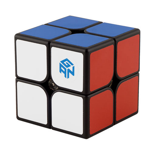
2x2

Smaller than the classic cube, this puzzle is much easier to solve, with the world record being under 1 second. There are several methods for solving the 2x2:

• Layer by layer – solve the first layer intuitively, then solve the second layer with algorithms similar to 3x3 OLL and PLL
• Ortega – solve a face (one side of the same color), orient the second layer, then finish the cube with a single algorithm
• EG – solve a face, then finish the cube with a single algorithm (this method uses 126 algorithms)

Top solvers use one-looking (see glossary), which allows them to solve this puzzle very quickly.

4x4

The 4x4 cube, also known as the Rubik's Revenge, introduces additional complexity compared to the 3x3 due to the lack of fixed center pieces and the presence of more edge and center pieces. This means centers must be solved first, and edge pieces must be paired before the cube can be solved like a 3x3.

The most common method for solving the 4x4 is Yau, which is a variant of the reduction method. The Yau method typically involves:

1. Solving two opposite centers
2. Pairing three cross edges
3. Solving the remaining centers
4. Pairing the remaining edges
5. Solving the cube as a 3x3

The standard reduction method involves solving all centers first, then pairing all edges, and finally solving the cube as a 3x3. The Yau method is generally faster and more efficient.

A unique challenge with the 4x4 is parity errors—situations that cannot occur on a 3x3. The two main parities are:

• PLL parity: When only two corner or two edge pieces are swapped.
• OLL parity: OLL parity: A situation where only one edge is incorrectly oriente.

These parities occur because the 4x4 has an even number of layers, which allows for move combinations not possible on odd-layered cubes. Handling the parity requires a special algorithm.

The reason why the parity happens is mathematically very interesting, but is out of scope for this paper.

5x5

More pieces mean more work and more time. The common method is reduction, consisting of these steps:

• Solving centers (center pieces have a single color; the goal is to arrange them correctly)
• Pairing edges (edges have two colors; pairing means putting matching edge pieces together)
• 3x3 stage (once centers and edges are solved, the puzzle is essentially reduced to a 3x3 (hence the name) and can be solved using only outer layer turns)

6x6

The common method is reduction, involving solving centers, pairing edges, and the 3x3 stage. Sounds familiar? That's right, this method is exactly the same as the method for 5x5.

There are some differences, mainly parity—the same thing that happens on 4x4. But the key parts of the method are the same.

7x7

As you might expect, the method used is reduction, just like the 5x5 and 6x6. Once you know how to solve the 5x5, you can solve cubes of any size—even a 15x15—the method remains the same.

The use of the same method will be important later, where we discuss the correlation across these events.

For both 6x6 and 7x7, the standard format is not average of 5 solves, but mean of 3 solves. This is to reduce the time required for the event, as larger cubes take significantly longer to solve.

Megaminx

The Megaminx is a dodecahedron-shaped puzzle with 12 faces, each a different color. The solving process is similar to the 3x3 cube, basically solving it layer by layer, and finishing with the top layer. The last layer requires more algorithms due to the increased number of pieces. More pieces mean more work, but also thanks to more faces, there is more freedom in moving pieces around, allowing more efficient solutions not possible on regular 3x3.

Skewb

The Skewb is a cube-shaped puzzle, but it turns around its corners rather than its faces. It has 8 corners and 6 center pieces. The solution is relatively simple, often requiring only a few algorithms. Most methods involve solving the top and bottom layer, then the remaining centers. One-looking is commonly used by top solvers.

Pyraminx

The Pyraminx is a tetrahedron-shaped puzzle with 4 faces. It has 4 tips, 4 centers, and 6 edges. One-looking is commonly used by top solvers thanks to the small amount of pieces.

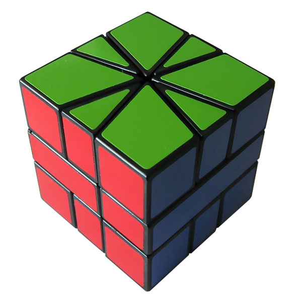
Square-1

Square-1 is a cube-shaped puzzle that can change shape as it is scrambled, making it a "shape-shifter". It's the only shape-shifting event in WCA competitions. It has 8 corners and 8 edges, but the pieces are not all the same size. The solution involves restoring the cube shape first, then solving the pieces. The puzzle requires unique algorithms due to its unusual mechanics and parity issues. The methods are overally algorithm-based, with very little room for intuitive solutions.

Rubik's clock

The only non-twisty puzzle in the WCA, Rubik's clock consists of 9 clocks on each side, each with a minute hand. The goal is to set all clocks to 12 o'clock. The puzzle is solved by switching pins and turning gears that affect multiple clocks simultaneously.

3x3 One Handed

The 3x3 One-Handed event is similar to the regular 3x3 event, but competitors must solve the cube using only one hand. The methods used are very similar to standard 3x3 solving.

Interesting fact: most right handed cubers use their left hand for one-handed solving.

Blindfolded events

Blindfolded events include 3x3 Blindfolded, 4x4 Blindfolded, 5x5 Blindfolded, and Multi-Blind. In these events, competitors memorize the puzzle during inspection, then solve it blindfolded. There is no inspection in these events and the the memorization part of the solve is included in the total solve time.

Methods used for blindfolded solving require lot more moves than traditional puzzle methods. They essentially solve the cube "piece by piece", while not moving any other pieces which aren't being solved at the time.

Multi-blind is about solving multiple differently scambled 3x3 cubes blindfolded–first memorizing all of them, then solving. The competitor can choose how many cubes they want to attempt to solve.

FMC (Fewest Moves Challenge)

In FMC, competitors are given a scramble and have 1 hour to find the solution using the fewest possible moves. It's the only event where time is not the goal.

---

Section 4: Goal of this statistical project, methodology, hypotheses

The goal is to measure the correlation between how good a person is at different speedcubing events.

To do this, we first need a way to quantify how "good" someone is at an event.

Measuring how "good" a speedcuber is at some event

There are two main approaches I came up with to quantify this. Let's go over them and list their properties, advantages and disadvantages.

1. Performance Ratio (Relative to World Record)
   • For each competitor, their best time divided by the world record time shows how many times they are slower than the record. This simple and intuitive metric which turns out to be quite effective and consistent across events.
   • This method is less affected by the popularity of the event, as it directly compares the competitor's performance to the best in the world.
   • Since FMC (3x3 Fewest moves) is an untimed event, this method doesn't make much sense to use for it.
   • This method will be called the "performance ratio" method from now on for simplicity.
2. Relative Ranking (Percentile)
   • There are world, continental and country rankings for each event. For simplicity, world ranking will be used, since it provides most amount of data.
   • Comparison of absolute rankings makes only little sense, since there are events with very different popularity–unsurprisingly, 3x3 is the event almost every competitor has participated in. In contrast, events like 5x5 blindfolded aren't as popular. This is because of their difficulty and the fact that not many competitions include them.
   • For the reasons stated above, percentile will be used.
   • This method will be called the "percentile" method from now on for simplicity.

For both approaches, the average of 5 solves will be compared, since it offers more balanced view of competitors ability. Single solves can be more based on luck, while averaging multiple solves also shows consistency of their skill.

If average of 5 can't be used (either due to lack of data, or due to event's different format), the best single solve will be used instead.

As I am unsure of which approach is better, I will calculate correlations using both.

My hypotheses

Based on my experience as a speedcuber, I have developed several hypotheses about the correlation between different events. A bit of context: I competed for the first time in Bratislava in 2016. My best 3x3 average is 11.68 seconds, ranking me 94th (out of 703) in the Czech Republic and about 15,000th (out of almost 250,000) competitors worldwide. You can also have a look at my WCA profile.

What correlations I expect

The correlation coefficion is denoted by $r$ in the following paragraph.

1. 5x5, 6x6, and 7x7 are solved using the same method, and improving times on them means improving very similar skills. Therefore, I expect those to be highly correlated.
   • These events are more "stamina-based" since they all take upwards of several minutes to complete the solve. This also adds to their similarity.
   • Hypothesis: strong positive correlation, $r\geq0.7$
2. 3x3 and 4x4 are very popular events many cubers practice together. While their methods differ a bit (4x4 adds several steps on top of the 3x3 method), I expect them to be quite correlated as well.
   • Hypothesis: strong positive correlation, $r\geq0.7$
3. 3x3 Blindfolded, 4x4 Blindfolded, and 5x5 Blindfolded I expect to have a low to moderate correlation with other non-blindfolded events, but a strong correlation with each other. Once a cuber finds blindfolded solving fun, they are probably willing to practice other blindfolded events too. There are also many cubers with good results in other events, but don't compete in blidfolded solving since they find it uninteresting.
   • Hypotheses:
     • moderate positive correlation, $0.4 \leq r \leq 0.6$ with other non blindfolded events
     • strong positive correlation, $r\geq0.7$ between each pair of blindfolded events
4. 3x3 Fewest Moves won't correlate with much with anything. It's a thing of its own, also because it's the only untimed event.
   • Hypothesis: weak positive correlation, $r \leq 0.3$ with all other events
5. Square-1 is a puzzle very different from all others. I expect the correlation to be quite moderate, but not very high since cubers who are generally more willing to practice in general will also practice Square-1, improving their times.
   • Hypothesis: moderate positive correlation, $0.4 \leq r \leq 0.6$ with all other events.
6. 2x2, Pyraminx, and Skewb are all fast-paced, short events. Top solvers usually use one-looking in all three. Their methods don't share many similarities, but many cubers I know practice them together. I expect decent correlation there.
   • Hypothesis: strong positive correlation, $r \geq 0.7$

Section 5: Calculating the correlations

Let's start by calculating the performance ratio correlations first.

# Compute correlation matrix for all events (Pearson correlation)
import numpy as np
from scipy.stats import pearsonr
import pandas as pd

results = pd.read_csv(
    'data/WCA_export_Results.tsv',
    sep='\t',
    dtype={'average': 'int', 'best': 'int'},
)
results['average'] = results['average'].fillna(0).astype(int)
results['best'] = results['best'].fillna(0).astype(int)

results['score'] = np.where(results['average'] > 0, results['average'], results['best'])

# Get best score for each person and event for ALL events
best_scores = results[results['score'] > 0].groupby(['personId', 'eventId'])['score'].min().reset_index()

# Get world record for each event (lowest score)
world_records = best_scores.groupby('eventId')['score'].min().to_dict()

# Compute performance ratio
best_scores['performance_ratio'] = best_scores.apply(
    lambda row: row['score'] / world_records[row['eventId']], axis=1
)

all_pivot = best_scores.pivot(index='personId', columns='eventId', values='performance_ratio')

# Filter events with enough data
min_competitors = 30
events_to_exclude = ['333mbf', '333mbo', 'magic', 'mmagic', '333ft']
valid_events = [eid for eid in all_pivot.columns if all_pivot[eid].count() >= min_competitors and eid not in events_to_exclude]

# Initialize correlation matrix for performance ratio
event_corr = pd.DataFrame(index=valid_events, columns=valid_events, dtype=float)

# Calculate correlation for each pair

for i, e1 in enumerate(valid_events):
    for j, e2 in enumerate(valid_events):
        if e1 == e2:
            event_corr.loc[e1, e2] = 1.0
        elif i > j:
            event_corr.loc[e1, e2] = event_corr.loc[e2, e1]  # Symmetric
        else:
            pair = all_pivot[[e1, e2]].dropna()
            if len(pair) >= min_competitors:
                try:
                    corr, _ = pearsonr(pair[e1], pair[e2])
                    event_corr.loc[e1, e2] = corr
                except ValueError:
                    event_corr.loc[e1, e2] = np.nan
            else:
                event_corr.loc[e1, e2] = np.nan

Now let's do the same, but using the percentile method this time.

# Calculate correlation matrix using world ranking percentile

ranks = pd.read_csv('data/WCA_export_RanksAverage.tsv', sep='\t', dtype=str)
ranks['worldRank'] = pd.to_numeric(ranks['worldRank'], errors='coerce')
event_counts = ranks.groupby('eventId')['personId'].count().to_dict()
ranks['percentile'] = ranks.apply(
    lambda row: 1 - (row['worldRank'] - 1) / event_counts[row['eventId']], axis=1
)

pivot_pct = ranks.pivot(index='personId', columns='eventId', values='percentile')
min_competitors = 30
events_to_exclude = ['333mbf', '333mbo', 'magic', 'mmagic', '333ft']
valid_events = [eid for eid in pivot_pct.columns if pivot_pct[eid].count() >= min_competitors and eid not in events_to_exclude]

# Ensure valid_events only contains eventIds present in pivot_pct columns
valid_events = [eid for eid in valid_events if eid in pivot_pct.columns]

# Initialize correlation matrix for percentile
event_corr_pct = pd.DataFrame(index=valid_events, columns=valid_events, dtype=float)

# Calculate correlation for each pair
for i, e1 in enumerate(valid_events):
    for j, e2 in enumerate(valid_events):
        if e1 == e2:
            event_corr_pct.loc[e1, e2] = 1.0
        elif i > j:
            event_corr_pct.loc[e1, e2] = event_corr_pct.loc[e2, e1]  # Symmetric
        else:
            if e1 not in pivot_pct.columns or e2 not in pivot_pct.columns:
                event_corr_pct.loc[e1, e2] = np.nan
                continue
            pair = pivot_pct[[e1, e2]].dropna()
            if len(pair) >= min_competitors:
                try:
                    corr, _ = pearsonr(pair[e1], pair[e2])
                    event_corr_pct.loc[e1, e2] = corr
                except ValueError:
                    event_corr_pct.loc[e1, e2] = np.nan
            else:
                event_corr_pct.loc[e1, e2] = np.nan

Here's the resulting correlation matrix for performance ratio, rounded to two decimal digits:

event_corr_rounded = event_corr.round(2)
display(event_corr_rounded)

	222	333	333bf	333fm	333oh	444	444bf	555	555bf	666	777	clock	minx	pyram	skewb	sq1
222	1.00	0.78	0.27	-0.02	0.68	0.69	0.20	0.62	0.15	0.54	0.48	0.38	0.57	0.57	0.58	0.47
333	0.78	1.00	0.31	-0.01	0.83	0.83	0.23	0.74	0.17	0.66	0.59	0.40	0.65	0.58	0.58	0.50
333bf	0.27	0.31	1.00	0.01	0.29	0.33	0.71	0.30	0.64	0.26	0.23	0.17	0.28	0.20	0.20	0.21
333fm	-0.02	-0.01	0.01	1.00	-0.01	-0.03	0.04	-0.02	0.02	0.01	-0.02	-0.02	-0.02	-0.01	-0.00	-0.02
333oh	0.68	0.83	0.29	-0.01	1.00	0.74	0.21	0.67	0.18	0.58	0.50	0.36	0.60	0.47	0.47	0.47
444	0.69	0.83	0.33	-0.03	0.74	1.00	0.24	0.85	0.20	0.77	0.69	0.40	0.70	0.53	0.51	0.52
444bf	0.20	0.23	0.71	0.04	0.21	0.24	1.00	0.22	0.83	0.23	0.21	0.15	0.18	0.17	0.11	0.16
555	0.62	0.74	0.30	-0.02	0.67	0.85	0.22	1.00	0.20	0.87	0.83	0.35	0.69	0.49	0.43	0.49
555bf	0.15	0.17	0.64	0.02	0.18	0.20	0.83	0.20	1.00	0.20	0.16	0.10	0.16	0.12	0.09	0.18
666	0.54	0.66	0.26	0.01	0.58	0.77	0.23	0.87	0.20	1.00	0.91	0.32	0.64	0.43	0.37	0.44
777	0.48	0.59	0.23	-0.02	0.50	0.69	0.21	0.83	0.16	0.91	1.00	0.27	0.61	0.41	0.33	0.42
clock	0.38	0.40	0.17	-0.02	0.36	0.40	0.15	0.35	0.10	0.32	0.27	1.00	0.44	0.45	0.45	0.39
minx	0.57	0.65	0.28	-0.02	0.60	0.70	0.18	0.69	0.16	0.64	0.61	0.44	1.00	0.57	0.53	0.52
pyram	0.57	0.58	0.20	-0.01	0.47	0.53	0.17	0.49	0.12	0.43	0.41	0.45	0.57	1.00	0.59	0.46
skewb	0.58	0.58	0.20	-0.00	0.47	0.51	0.11	0.43	0.09	0.37	0.33	0.45	0.53	0.59	1.00	0.44
sq1	0.47	0.50	0.21	-0.02	0.47	0.52	0.16	0.49	0.18	0.44	0.42	0.39	0.52	0.46	0.44	1.00

And here's the matrix for the percentile method, also rounded:

event_corr_pct_rounded = event_corr_pct.round(2)
display(event_corr_pct_rounded)

	222	333	333bf	333fm	333oh	444	444bf	555	555bf	666	777	clock	minx	pyram	skewb	sq1
222	1.00	0.88	0.19	0.36	0.66	0.67	0.17	0.55	0.24	0.46	0.39	0.51	0.53	0.73	0.69	0.50
333	0.88	1.00	0.24	0.39	0.78	0.78	0.20	0.67	0.33	0.57	0.50	0.48	0.58	0.68	0.66	0.50
333bf	0.19	0.24	1.00	0.28	0.22	0.24	0.73	0.22	0.66	0.21	0.16	0.19	0.20	0.16	0.14	0.21
333fm	0.36	0.39	0.28	1.00	0.45	0.41	0.19	0.40	0.20	0.38	0.33	0.22	0.37	0.29	0.30	0.35
333oh	0.66	0.78	0.22	0.45	1.00	0.76	0.12	0.67	0.19	0.56	0.48	0.41	0.60	0.50	0.50	0.51
444	0.67	0.78	0.24	0.41	0.76	1.00	0.20	0.85	0.25	0.74	0.67	0.44	0.67	0.51	0.51	0.54
444bf	0.17	0.20	0.73	0.19	0.12	0.20	1.00	0.17	0.85	0.15	0.11	0.10	0.11	0.14	0.09	0.16
555	0.55	0.67	0.22	0.40	0.67	0.85	0.17	1.00	0.29	0.88	0.82	0.39	0.66	0.42	0.41	0.51
555bf	0.24	0.33	0.66	0.20	0.19	0.25	0.85	0.29	1.00	0.23	0.26	0.12	0.16	0.23	0.23	0.25
666	0.46	0.57	0.21	0.38	0.56	0.74	0.15	0.88	0.23	1.00	0.93	0.36	0.62	0.36	0.37	0.47
777	0.39	0.50	0.16	0.33	0.48	0.67	0.11	0.82	0.26	0.93	1.00	0.30	0.56	0.31	0.32	0.43
clock	0.51	0.48	0.19	0.22	0.41	0.44	0.10	0.39	0.12	0.36	0.30	1.00	0.43	0.52	0.53	0.47
minx	0.53	0.58	0.20	0.37	0.60	0.67	0.11	0.66	0.16	0.62	0.56	0.43	1.00	0.47	0.48	0.53
pyram	0.73	0.68	0.16	0.29	0.50	0.51	0.14	0.42	0.23	0.36	0.31	0.52	0.47	1.00	0.69	0.46
skewb	0.69	0.66	0.14	0.30	0.50	0.51	0.09	0.41	0.23	0.37	0.32	0.53	0.48	0.69	1.00	0.49
sq1	0.50	0.50	0.21	0.35	0.51	0.54	0.16	0.51	0.25	0.47	0.43	0.47	0.53	0.46	0.49	1.00

For technical reasons, event names from the WCA dataset don't exactly match their full names. Refer to the following table for their full names:

Event name in dataset	Full event name
222	2x2 cube
333	3x3 cube
333bf	3x3 blindfolded
333oh	3x3 one-handed
444	4x4 cube
444bf	4x4 blindfolded
555	5x5 cube
555bf	5x5 blindfolded
666	6x6 cube
777	7x7 cube
clock	Rubik's clock
minx	Megaminx
pyram	Pyraminx
skewb	Skewb
sq1	Square-1

Let's use a heatmap for better visualisation:

import seaborn as sb

import matplotlib.pyplot as plt

plt.figure(figsize=(12, 10))
sb.heatmap(event_corr_pct_rounded, annot=True, cmap='coolwarm', vmin=0, vmax=1, linewidths=0.5)
plt.title('Correlation Heatmap (Percentile Method)')
plt.ylabel('Event')
plt.xlabel('Event')
plt.tight_layout()
plt.show()

Section 6: Results interpretation

For supporting or rejecting my hypothesis, I will only use results provided by the "relative ranking/percentile" method, since I believe it's more consistent across events.

Hypothesis 1: 5x5, 6x6 and 7x7

Expectation: $r\geq0.7$

Let's have a look at correlation between "big cubes":

display(event_corr_pct_rounded.loc[['555', '666', '777'], ['555', '666', '777']])

	555	666	777
555	1.00	0.88	0.82
666	0.88	1.00	0.93
777	0.82	0.93	1.00

The data supports the hypothesis, all three pairs of events have a correlation of $\geq 0.8$, showing a significant positive correlation.

Hypothesis 2: 3x3 and 4x4

Expectation: $r\geq0.7$

display(event_corr_pct_rounded.loc[['333'], ['444']])

	444
333	0.78

Again, hypothesis is supported by the data, the correlation is 0.78.

Hypothesis 3: Blindfolded events

Expectation:

• $0.4 \leq r \leq 0.6$ with other non blindfolded events
• $r\geq0.7$ between each pair of blindfolded events

Let's look at correlations of 3x3-5x5 blindfolded with other events:

blind_events = ['333bf', '444bf', '555bf']
other_events = [col for col in event_corr_pct_rounded.columns if col not in blind_events]
display(event_corr_pct_rounded.loc[blind_events, other_events])

	222	333	333fm	333oh	444	555	666	777	clock	minx	pyram	skewb	sq1
333bf	0.19	0.24	0.28	0.22	0.24	0.22	0.21	0.16	0.19	0.20	0.16	0.14	0.21
444bf	0.17	0.20	0.19	0.12	0.20	0.17	0.15	0.11	0.10	0.11	0.14	0.09	0.16
555bf	0.24	0.33	0.20	0.19	0.25	0.29	0.23	0.26	0.12	0.16	0.23	0.23	0.25

We can observe low poitive correlations with other events, with all being < 0.3, so the hypothesis was in fact incorrect.

Let's take a look at correlations among blindfolded events:

display(event_corr_pct_rounded.loc[['333bf', '444bf', '555bf'], ['333bf', '444bf', '555bf']])

	333bf	444bf	555bf
333bf	1.00	0.73	0.66
444bf	0.73	1.00	0.85
555bf	0.66	0.85	1.00

Now the correlations aren't low at all, with the highest being between 4x4 BLD and 5x5 BLD—which is not surprising, since both events require very similar skills and use practically the same method.

The hypothesis was correct for 3x3 blindfolded–4x4 blindfolded and 4x4 blindfolded–5x5 blindfolded, but incorrect for 3x3 blindfolded–5x5 blindfolded.

3x3 blindfolded has a slightly lower correlation with both 4x4 and 5x5 blindfolded, though it's still much higher than with other events. Again, this is not very surprising, and I believe the lower number can be explained by the lower popularity of 4x4 and 5x5 blindfolded. The popularity of events is discussed further below in Section 6.

Hypothesis 4: 3x3 fewest moves

Expectation: $r\lt 0.3$ with other events.

This time, we'll review both the performance ratio and percentile method correlations, since they differ quite a bit.

Let's examine the correlation between 3x3 Fewest Moves (FMC) and other events using the performance ratio method:

display(event_corr_rounded.loc[['333fm']])

	222	333	333bf	333fm	333oh	444	444bf	555	555bf	666	777	clock	minx	pyram	skewb	sq1
333fm	-0.02	-0.01	0.01	1.0	-0.01	-0.03	0.04	-0.02	0.02	0.01	-0.02	-0.02	-0.02	-0.01	-0.0	-0.02

Rounded down, it shows zero correlation with other events.

Now let's have a look at correlation using the percentile method:

display(event_corr_pct_rounded.loc[['333fm']])

	222	333	333bf	333fm	333oh	444	444bf	555	555bf	666	777	clock	minx	pyram	skewb	sq1
333fm	0.36	0.39	0.28	1.0	0.45	0.41	0.19	0.4	0.2	0.38	0.33	0.22	0.37	0.29	0.3	0.35

These percentile-based correlations for FMC are noticeably higher (≈0.2–0.4) than when using performance ratios. The primary cause for this is probably the fact that the performance ratio for FMC doesn't compare solve times unlike other events, so the reliablility of the ratio for this event is questionable.

Hypothesis was therefore correct if using the performace ratio, but incorrect for percentile method.

Hypothesis 5: Square-1

Expectation: $0.4 \leq r \leq 0.6$ with all other events.

display(event_corr_pct_rounded.loc[['sq1']])

	222	333	333bf	333fm	333oh	444	444bf	555	555bf	666	777	clock	minx	pyram	skewb	sq1
sq1	0.5	0.5	0.21	0.35	0.51	0.54	0.16	0.51	0.25	0.47	0.43	0.47	0.53	0.46	0.49	1.0

Overall, the correlation for Square-1 with other events ranges from 0.4 to 0.6, with the exception of blindfolded events and 3x3 Fewest Moves, which—as previously demonstrated—show consistently low correlations. This outcome aligns with expectations and supports the hypothesis.

Hypothesis 6: 2x2, Skewb and Pyraminx

Expectation: $r\geq 0.7$ between each pair of events.

display(event_corr_pct_rounded.loc[['222', 'skewb', 'pyram'], ['222', 'skewb', 'pyram']])

	222	skewb	pyram
222	1.00	0.69	0.73
skewb	0.69	1.00	0.69
pyram	0.73	0.69	1.00

The data supports the hypothesis, with the skewb–pyraminx correlation at 0.69, which is very close to 0.7. In practical terms, a correlation of 0.69 indicates a strong positive relationship between the two events—just shy of the threshold set in the hypothesis. Given the variability in competitor skill and event participation, this result can reasonably be interpreted as supporting the hypothesis.

Section 7: Other interesting data

Let's explore additional insights from the WCA dataset.

To start, we'll examine the popularity of each event by counting how many competitors have participated in them. This will give us a clear ranking of event popularity within the speedcubing community:

# List all events from valid_events and display the total number of competitors, sorted by popularity
event_popularity = {eid: all_pivot[eid].count() for eid in valid_events}
event_popularity_sorted = sorted(event_popularity.items(), key=lambda x: x[1], reverse=True)

total_competitors = all_pivot.index.nunique()

print(f"Total number of distinct competitors: {total_competitors:,}")
event_popularity_df = pd.DataFrame(event_popularity_sorted, columns=['eventId', 'num_competitors'])
event_popularity_df['percent_of_competitors'] = (
    pd.to_numeric(event_popularity_df['num_competitors']) / total_competitors * 100
).round(2).astype(str) + ' %'
event_popularity_df_v = event_popularity_df.copy()
event_popularity_df_v['num_competitors'] = event_popularity_df_v['num_competitors'].map('{:,}'.format)
display(event_popularity_df_v.style.hide(axis='index'))

Total number of distinct competitors: 268,229

eventId	num_competitors	percent_of_competitors
333	258,078	96.22 %
222	170,130	63.43 %
pyram	117,934	43.97 %
444	76,460	28.51 %
333oh	67,171	25.04 %
skewb	66,653	24.85 %
555	37,009	13.8 %
minx	31,047	11.57 %
clock	26,979	10.06 %
sq1	22,885	8.53 %
666	15,465	5.77 %
777	12,447	4.64 %
333fm	11,298	4.21 %
333bf	11,033	4.11 %
444bf	1,961	0.73 %
555bf	1,014	0.38 %

Let's visualise this in a graph:

# Prepare event popularity DataFrame with "All" row on top
event_pop_df_simple = event_popularity_df.copy()
event_pop_df_simple['percent'] = (
    pd.to_numeric(event_pop_df_simple['num_competitors']) / total_competitors * 100
).round(2)
all_row = pd.DataFrame([{'eventId': 'All', 'num_competitors': total_competitors, 'percent': 100.0}])
event_pop_df_simple = pd.concat([all_row, event_pop_df_simple], ignore_index=True)

plt.figure(figsize=(9, 6))
sb.barplot(
    data=event_pop_df_simple,
    x='num_competitors',
    y='eventId',
    order=event_pop_df_simple['eventId']
)
plt.title('Event popularity — number of distinct competitors')
plt.xlabel('Number of competitors')
plt.ylabel('Event')

for idx, row in event_pop_df_simple.iterrows():
    plt.text(row['num_competitors'] * 1.01, idx,
             f"{int(row['num_competitors']):,} ({row['percent']:.2f}%)",
             va='center', fontsize=9)

plt.xlim(0, event_pop_df_simple['num_competitors'].max() * 1.2)
plt.tight_layout()
plt.show()

It's no surprise that nearly every speedcuber participates in the 3x3 event. However, there are a few exceptions—almost 4% of competitors have never competed in 3x3. What events do these speedcubers choose instead? Below is a list of events along with the number of competitors who have never competed in 3x3:

# Find competitors who have NOT competed in 3x3
no_333 = all_pivot[all_pivot['333'].isna()]

# For these competitors, count how many have a non-null result in each event (excluding 333)
event_counts_no_333 = no_333.drop(columns=['333']).notna().sum().sort_values(ascending=False)

# Display as a DataFrame for readability
event_counts_no_333_df = event_counts_no_333.reset_index()
event_counts_no_333_df.columns = ['eventId', 'num_competitors']
display(event_counts_no_333_df.style.hide(axis='index'))

eventId	num_competitors
222	5068
pyram	5064
skewb	1155
clock	573
444	530
magic	310
minx	295
333oh	292
555	240
333bf	161
sq1	156
666	78
333fm	77
777	68
mmagic	68
333mbf	42
444bf	31
555bf	15
333ft	5
333mbo	3

Let's visualise it in a graph:

# Plot a horizontal bar chart for better visualization
plt.figure(figsize=(8, 6))
sb.barplot(
    data=event_counts_no_333_df,
    y='eventId',
    x='num_competitors',
)
plt.title('Event Participation of Competitors Who Never Competed in 3x3')
plt.xlabel('Number of Competitors')
plt.ylabel('Event')
plt.tight_layout()
plt.show()

The results are unsurprising—the top three events favored by competitors who haven't participated in 3x3 are generally regarded as easier than the 3x3 cube.

Disclaimer

This information is based on competition results owned and maintained by the World Cube Association, published at https://worldcubeassociation.org/results as of September 16, 2025.